


5. Performance analysis
- 5.1 Performance Analysis Tools
- 5.2 Cray Performance Analysis Tool (CrayPat)
- 5.3 Cray Reveal
- 5.4 MAP Profiler (Arm Forge)
- 5.5 Tuning and Analysis Utilities (TAU)
- 5.6 Valgrind
- 5.7 General hints for interpreting profiling results
This section covers the use of tools on ARCHER to analyse the performance of your code, both in terms of the serial performance (percentage of peak, memory usage, etc.) and in terms of the parallel performance (load balance, time in MPI routines, etc.).
There are a number of tools installed on ARCHER available to help you understand the performance characteristics of your code and some will even offer suggestions on how to improve performance.
5.1 Performance Analysis Tools
These tools include
- Cray Performance Analysis Tool (CrayPat)
- Arm MAP
- TAU
- Valgrind
5.2 Cray Performance Analysis Tool (CrayPat)
CrayPat consists of two command line tools which are used to profile your code
pat_buildadds instrumentation to your code so that when you run the instrumented binary the profiling information is stored on disk;pat_reportreads the profiling information on disk and compiles it into human-readable reports.
The analysis produced by pat_report can be visualised using
the Cray Apprentice2 tool app2.
CrayPat can perform two types of performance analysis: sampling experiments and tracing experiments. A sampling experiment probes the code at a predefined interval and produces a report based on these statistics. A tracing experiment explicitly monitors the code performance within named routines. Typically, the overhead associated with a tracing experiment is higher than that associated with a sampling experiment but provides much more detailed information. The key to getting useful data out of a sampling experiment is to run your profiling for a representative length of time.
Detailed documentation on CrayPat is available from Cray. The latest version of the documentation can be found at the top of this list:
5.2.1 Instrumenting a code with pat_build
Often the best way to to analyse the performance is to run a sampling experiment and then use the results from this to perform a focused tracing experiment. CrayPat contains the functionality for automating this process - known as Automatic Profiling Analysis (APA).
The example below illustrates how to do this.
5.2.1.1 Example: Profiling the CASTEP Code
Here is a step-by-step example of instrumenting and profiling the performance of a code (CASTEP) using CrayPat.
The first step is to compile your code with the profiling tools
attached. First load the Cray perftools-base module with
module load perftools-base
then, you can load the Cray perftools module with
module load perftools.
Next, compile the CASTEP code in the standard way on
the /work file-system (which is accessible on the compute
nodes). Once you have the CASTEP executable you need to instrument
it for a sampling experiment. The following command will
produce the castep+samp instrumented executable
pat_build -o castep+samp castep
The default instrumentation is a sampling experiment with Automatic
Profiling Analysis (equivalent to the option -O apa).
Run your instrumented program as you usually would in the job submission system at your site. For example
#!/bin/bash --login
#PBS -N castep_profile
#PBS -l select=32
#PBS -l walltime=1:00:00
# Replace [budget code] below with your project code
#PBS -A [budget code]

# Make sure any symbolic links are resolved to absolute path
export PBS_O_WORKDIR=$(readlink -f $PBS_O_WORKDIR)
# Change to the directory that the job was submitted from
cd $PBS_O_WORKDIR

# Run the sampling experiment
aprun -n 768 castep+samp input
When the job completes successfully the directory you submitted the
job from will either contain a .xf file (if you used a
small number of cores) with a name
like castep+samp+25370-14s.xf or a directory (for large
core counts) with a name like castep+samp+25370-14s.
The actual name is dependent on the name of your instrumented
executable and the process ID. In this case we used 32 nodes so we
have a directory.
The next step is to produce a basic performance report and also the
Automatic Profiling Analysis input for pat_build to create
a tracing experiment. This is done (usually interactively) by using
the pat_report command (you must have
the perftools module loaded to use the pat_report
command). In our example we would type
pat_report -o castep_samp_1024.pat castep+samp+25370-14s
This will produce a text report (in this
case, castep_samp_1024.pat) listing the various routines in
the program and how much time was spent in each one during the run
(see below for a discussion on the contents of this file). It also
produces a castep+samp+25370-14s.ap2 file and
a castep+samp+25370-14s.apa file.
-
The
.ap2file can be used with the Cray Apprentice2 visualisation tool to get an alternative view of the code performance. -
The
.apafile can be used as the input topat_buildto produce a tracing experiment focused on the routines that take most time (as determined in the previous sampling experiment). We illustrate this below.
An .apa file may not be produced if the program is very
short, or mainly calls library functions, with little processing in
the program itself. There will be a message at the end of the text
report like
    No .apa file with pat_build option suggestions was generated
    because no samples appear to have been taken in USER functions.
For information on interpreting the results in the sampling experiment text report, see the section below.
To produce a focused tracing experiment based on the results from
the sampling experiment above we would use the pat_build
command with the .apa file produced above. (Note, there
is no need to change directory to the directory containing the
original binary to run this command.)
pat_build -O castep+samp+25370-14s.apa -o castep+apa
This will generate a new instrumented version of the CASTEP
executable (castep+apa) in the current working directory.
You can then submit a job (as outlined above) making sure that you
reference this new executable. This will then run a tracing
experiment based on the options in the .apa file.
Once again, you will find that your job generates a .xf
file (or a directory) which you can analyse using
the pat_report command. Please see the section below for
information on analysing tracing experiments.
5.2.2 Analysing profile results using pat_report
The pat_report command is able to produce many
different profile reports from the profile data. You can select a
predefined report with the -O flag
to pat_report. A selection of the most generally
useful predefined report types are
-
ca+src- Show the callers (bottom-up view) leading to the routines that have a high use in the report and include source code line numbers for the calls and time-consuming statements. -
load_balance- Show load-balance statistics for the high-use routines in the program. Parallel processes with minimum, maximum and median times for routines will be displayed. Only available with tracing experiments. -
mpi_callers- Show MPI message statistics. Only available with tracing experiments.
Multiple options can be specified to the -O flag if they
are separated by commas. For example
pat_report -O ca+src,load_balance -o castep_furtherinfo_1024.pat castep+samp+25370-14s
You can also define your own custom reports using the -b
and -d flags to pat_report. Details on how to do
this can be found in the pat_report documentation and man
pages. The output from the predefined report types (described
above) show the settings of the -b and -d flags
that were used to generate the report. You can use these examples
as the basis for your own custom reports.
Below, we show examples of the output from sampling and tracing experiments for the pure MPI version of CASTEP. A report from your own code will differ in the routines and times shown. Also, if your code uses OpenMP threads, SHMEM, or CAF/UPC then you will also see different output.
5.2.2.1 Example: results from a sampling experiment on CASTEP
In a sampling experiment, the main summary table produced
by pat_report will look something like (of course, your
code will contain different functions and subroutines)
Table 1:  Profile by Function

   Samp%  |  Samp  |  Imb.  |  Imb.  |Group
          |        |  Samp  | Samp%  | Function
          |        |        |        |  PE=HIDE

   100.0% | 6954.6 |     -- |     -- |Total
|------------------------------------------------------------------------
|   46.0% | 3199.8 |     -- |     -- |MPI
||-----------------------------------------------------------------------
||  12.9% |  897.0 |  302.0 |  25.6% |mpi_bcast
||  12.9% |  896.4 |   78.6 |   8.2% |mpi_alltoallv
||   8.7% |  604.2 |  139.8 |  19.1% |MPI_ALLREDUCE
||   5.4% |  378.6 | 1221.4 |  77.5% |MPI_SCATTER
||   4.9% |  341.6 |  320.4 |  49.2% |MPI_BARRIER
||   1.1% |   75.8 |  136.2 |  65.2% |mpi_gather
||=======================================================================
|   38.8% | 2697.9 |     -- |     -- |USER
||-----------------------------------------------------------------------
||   9.4% |  652.1 |  171.9 |  21.2% |comms_transpose_exchange.3720
||   6.0% |  415.2 |   41.8 |   9.3% |zgemm_kernel_n
||   3.4% |  237.6 |   29.4 |  11.2% |zgemm_kernel_l
||   3.1% |  215.6 |   24.4 |  10.3% |zgemm_otcopy
||   1.7% |  119.8 |   20.2 |  14.6% |zgemm_oncopy
||   1.3% |   92.3 |   11.7 |  11.4% |zdotu_k
||=======================================================================
|   15.2% | 1057.0 |     -- |     -- |ETC
||-----------------------------------------------------------------------
||   2.0% |  140.5 |   32.5 |  19.1% |__ion_MOD_ion_q_recip_interpolation
||   2.0% |  139.8 |  744.2 |  85.5% |__remainder_piby2
||   1.1% |   78.3 |   32.7 |  29.9% |__ion_MOD_ion_apply_and_add_ylm
||   1.1% |   73.5 |   35.5 |  33.1% |__trace_MOD_trace_entry
|========================================================================
You can see that CrayPat splits the results from a sampling experiment into three sections
- MPI - samples accumulated in message passing routines
- USER - samples accumulated in user routines. These are usually the functions and subroutines that are part of your program.
- ETC - samples accumulated in library routines.
The first two columns indicate the percentage and number of samples
(mean of samples computed across all parallel tasks) and indicate
the functions in the program where the sampling experiment spent the
most time. Columns 3 and 4 give an indication of the differences
between the minimum number of samples and maximum number of samples
found across different parallel tasks. This, in turn, gives an
indication of where the load-imbalance in the program is found. It
may be that load imbalance is found in routines where insignificant
amounts of time are spent. In this case, the load-imbalance may not
actually be significant (for example, the large imbalance time seen
in mpi_gather in the example above.
In the example above - the largest amounts of time seem to be spent
in the MPI routines MPI_BCAST, MPI_ALLTOALLV
and MPI_ALLREDUCE; in the program
routine comms_transpose_exchange; and in the LAPACK
routine zgemm.
To narrow down where these time consuming calls are in the program
we can use the ca+src report option to pat_report
to get a view of the split of samples between the different calls to
the time consuming routines in the program.
pat_report -O ca+src -o castep_calls_1024.pat castep+samp+25370-14s
An extract from the the report produced by the above command looks like
Table 1:  Profile by Function and Callers, with Line Numbers

    Samp%  |  Samp  |Group
           |        | Function
           |        |  Caller
           |        |   PE=HIDE

    100.0% | 6954.6 |Total
|--------------------------------------------------------------------------------------
--snip--
|    38.8% | 2697.9 |USER
||-------------------------------------------------------------------------------------
||    9.4% |  652.1 |comms_transpose_exchange.3720
|||------------------------------------------------------------------------------------
3||   3.7% |  254.4 |__comms_MOD_comms_transpose_n:comms.mpi.F90:line.17965
4||        |        | __comms_MOD_comms_transpose:comms.mpi.F90:line.17826
5||        |        |  __fft_MOD_fft_3d:fft.fftw3.F90:line.482
6||   3.1% |  215.0 |   __basis_MOD_basis_real_recip_reduced_one:basis.F90:line.4104
7||        |        |    _s_wave_MOD_wave_real_to_recip_wv_bks:wave.F90:line.24945
8||        |        |     __pot_MOD_pot_nongamma_apply_wvfn_slice:pot.F90:line.2640
9||        |        |      __pot_MOD_pot_apply_wvfn_slice:pot.F90:line.2550
10|        |        |       __electronic_MOD_electronic_apply_h_recip_wv:electronic.F90:line.4364
11|        |        |        __electronic_MOD_electronic_apply_h_wv:electronic.F90:line.4057
12|   3.0% |  211.4 |         __electronic_MOD_electronic_minimisation:electronic.F90:line.1957
13|   3.0% |  205.6 |          __geometry_MOD_geom_get_forces:geometry.F90:line.6299
14|   2.8% |  195.2 |           __geometry_MOD_geom_bfgs:geometry.F90:line.2199
15|        |        |            __geometry_MOD_geometry_optimise:geometry.F90:line.1051
16|        |        |             MAIN__:castep.f90:line.1013
17|        |        |              main:castep.f90:line.623
--snip--
This indicates that (in the USER routines) the part of the
comms_transpose_exchange routine in which the program is
spending most time is around line 3720 (in many cases the
time-consuming line will be the start of a loop). Furthermore, we
can see that approximately one third of the samples in the routine
(3.7%) are originating from the call
to comms_transpose_exchange in the stack shown. Here, it
looks like they are part of the geometry optimisation section of
CASTEP. The remaining two-thirds of the time will be indicated
further down in the report.
In the original report we also get a table reporting on the wall clock time of the program. The table reports the minimum, maximum and median values of wall clock time from the full set of parallel tasks. The table also lists the maximum memory usage of each of the parallel tasks
Table 3:  Wall Clock Time, Memory High Water Mark

    Process  |  Process  |PE=[mmm]
       Time  |    HiMem  |
             | (MBytes)  |

  124.409675 |   100.761 |Total
|---------------------------------
| 126.922418 |   101.637 |pe.39
| 124.329474 |   102.336 |pe.2
| 122.241495 |   101.355 |pe.4
|=================================
If you see a very large difference in the minimum and maximum wall clock time for different parallel tasks it indicates that there is a large amount of load-imbalance in your code and it should be investigated more thoroughly.
5.2.2.2 Example: results from a tracing experiment on CASTEP
To be added.
5.2.3 Using hardware counters
CrayPat can also provide performance counter data during tracing
experiments. The PAT_RT_PERFCTR environment variable
can be set in your job script to specify hardware, network, and
power management events to be monitored. Please refer to the
CrayPat manpage and
the CrayPat documentation for information about using the performance counters.
5.2.3.1 Example: Performance counter results from CASTEP
To be added.
5.3 Cray Reveal
Reveal is a performance analysis tool supported by Cray that guides you in improving the performance of a Cray-compiled application code. Specifically, Reveal will analyse the loops within your code and identify which ones are less than fully optimised and why. In addition, Reveal can gather performance statistics that rank the loops according to execution time, thereby showing you the best places in the source code to apply optimisations. An overview of Reveal can be found in the Cray document entitled, Using Cray Performance Measurement and Analysis Tools. In addition, the ARCHER CSE team have produced a Reveal screencast (see below) that gives a straightforward example of how a researcher might run Reveal with their MPI application code, and, along the way, show how to make the code run faster, and also, how to add parallelism by introducing OpenMP directives. Further details on the OpenMP-aspects of the Reveal tool can be found in this Cray webinar.
5.4 MAP Profiler (Arm Forge)
MAP can be used to profile MPI code only - it does not support detailed profiling of OpenMP, SHMEM, CAF, or UPC. Profiling using MAP consists of four steps
- Create a MAP profiling version of your MPI library.
- Re-compile your code, linking to the MAP MPI profiling library.
- Run your code to collect profiling information.
- Visualise the profiling information using the MAP Remote Client.
5.4.1 Create a MAP profiling MPI library
You should first load the forge
module to give you access to all the MAP executables
module load forge
The command you use to create the profiling version of your MPI library differs depending whether you are linking statically or dynamically. On ARCHER the default is to link statically so you should use the command for static libraries unless you are definitely linking dynamically.
For statically linked applications the command is
make-profiler-libraries and you need to supply a
directory for the library files. For example, for user mjf
mjf@eslogin008:/work/z01/z01/mjf/test> mkdir map-libraries-static
mjf@eslogin008:/work/z01/z01/mjf/test> make-profiler-libraries --lib-type=static ./map-libraries-static
Creating Cray static libraries in /fs3/z01/z01/mjf/test/map-libraries-static
Detected ld version >= 2.25 (2.26.0.20160224)
Created the libraries:
   libmap-sampler-binutils-2.25.a
   libmap-sampler-pmpi.a

To instrument a program, add these compiler options:
   compilation for use with MAP - not required for Performance Reports:
      -g (or '-G2' for native Cray Fortran) (and -O3 etc.)
   linking (both MAP and Performance Reports):
      -Wl,@/fs3/z01/z01/mjf/test/map-libraries-static/allinea-profiler.ld ... EXISTING_MPI_LIBRARIES
   If your link line specifies EXISTING_MPI_LIBRARIES (e.g. -lmpi), then
   these must appear *after* the Allinea sampler and MPI wrapper libraries in
   the link line.  There's a comprehensive description of the link ordering
   requirements in the 'Preparing a Program for Profiling' section of either
   userguide-forge.pdf or userguide-reports.pdf, located in
   /home/y07/y07/cse/forge/19.0.1/doc/.
If you are linking dynamically then you still use the "make-profiler-libraries" command, but don't specify static building. For example
mjf@eslogin008:/work/z01/z01/mjf/test> mkdir map-libraries-dynamic
mjf@eslogin008:/work/z01/z01/mjf/test> make-profiler-libraries ./map-libraries-dynamic
Creating Cray shared libraries in /fs3/z01/z01/mjf/test/map-libraries-dynamic
Created the libraries:
   libmap-sampler.so       (and .so.1, .so.1.0, .so.1.0.0)
   libmap-sampler-pmpi.so  (and .so.1, .so.1.0, .so.1.0.0)

To instrument a program, add these compiler options:
   compilation for use with MAP - not required for Performance Reports:
      -g (or '-G2' for native Cray Fortran) (and -O3 etc.)
   linking (both MAP and Performance Reports):
      -dynamic -L/fs3/z01/z01/mjf/test/map-libraries-dynamic -lmap-sampler-pmpi -lmap-sampler -Wl,--eh-frame-hdr -Wl,-rpath=/fs3/z01/z01/mjf/test/map-libraries-dynamic

Note: These libraries must be on the same NFS/Lustre/GPFS filesystem as your
program.
When using dynamic linking, before running your program, set LD_LIBRARY_PATH:
export LD_LIBRARY_PATH=./map-libraries-dynamic:$LD_LIBRARY_PATH
or add -Wl,-rpath=./map-libraries-dynamic when linking your program.
5.4.2 Re-compile the code, linking to the MAP MPI libraries
Recompile your code with the -g flag (-G2
can be used with Cray Fortran) to ensure debugging information is
available for the profiler. Then link using the set of options
specified in the output from
the make-profiler-libraries command that you
used (note, the -lWl,@.... statement should be added at the end of command for linking the executable, not the beginning).
5.4.3 Run the code to collect profiling information
You can now run a job as normal to collect the profile information for your code. This involves writing a job submission script to run your code through MAP. MAP will produce a file containing all the profiling information which can then be examined using the Remote Client (as described below).
An example job submission script for running a profile across 24 MPI processes would be
#!/bin/bash --login
#
#PBS -N map_test
#PBS -l select=1
#PBS -l walltime=1:0:0
#PBS -A t01

cd $PBS_O_WORKDIR

module load forge

map -profile aprun -n 24 myapp.exe
This will produce a profile file with a name like
myapp_24p_2014-04-15-07.map
An example job submission script for running a profile across 24 MPI processes with 12 processes per node would be
#!/bin/bash --login
#
#PBS -N map_test
#PBS -l select=2
#PBS -l walltime=1:0:0
#PBS -A t01

cd $PBS_O_WORKDIR

module load forge

map -profile aprun -n 24 -N 12 -S 6 myapp.exe
You can specify a specific name for this output file using
the -output option to map in the job
script.
If you are profiling a dynamically linked program, then you will
need to set LD_LIBRARY_PATH in the job script.
5.4.4 Visualise the profiling information
In order to visualise the data you should download and install Arm Forge Remote Client on your desktop using these instructions.
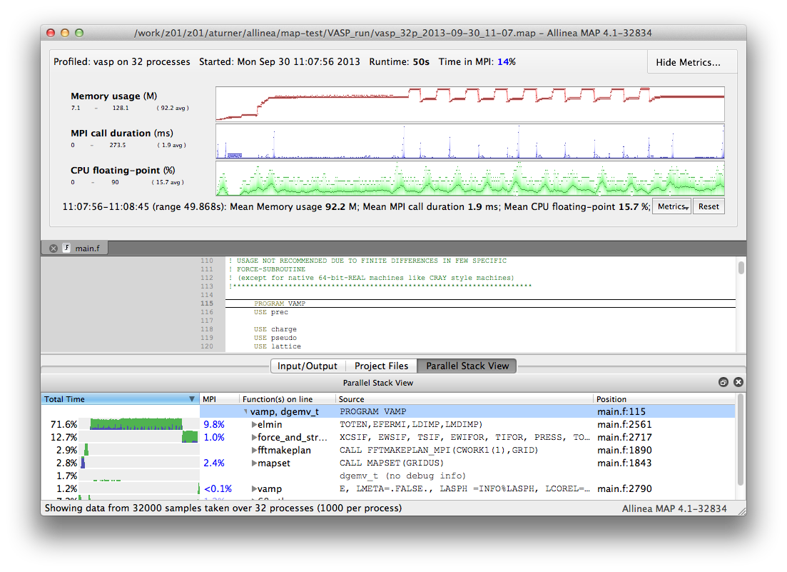
Once remote access has been successfully setup you should be returned to the startup screen. This time select "Load Profile Data File". You will be given a dialogue box where you can select your profile file from the ARCHER file-system. Once you have selected your file MAP will assemble your results and you can visualise your profile data. The MAP interface should look something like (this is for an older version of Forge):
For more information on using the profiling interface see:
5.5 Tuning and Analysis Utilities (TAU)
TAU is a portable profiling and tracing toolkit for performance analysis of parallel programs written in Fortran, C, C++, UPC, Java, Python. The current version of TAU installed on ARCHER is v2.25.1.1, the following makefiles are supported.
- Makefile.tau-cray-mpi-pdt
- Makefile.tau-cray-mpi-pdt-scorep
- Makefile.tau-cray-mpi-python-pdt
- Makefile.tau-cray-ompt-mpi-pdt-openmp
- Makefile.tau-cray-papi-mpi-pdt
- Makefile.tau-cray-papi-ompt-mpi-pdt-openmp Equivalent makefiles also exist for gnu and Intel programming environments.
Choose one of the makefiles and insert "export TAU_MAKEFILE=$TAU_LIB/" before compiling your code. Otherwise, use tau_exec for uninstrumented code.
Note, before using tau_exec, make sure you have built your application binary with the -dynamic link option. This is necessary because tau_exec preloads a dynamic shared object, libTAU.so, in the context of the executing application.
Full documentation can be found at http://www.cs.uoregon.edu/research/tau/docs.php. In addition, TAU workshop exercises can be found at /home/y07/shared/tau/workshop/ - please start with the readme file located within the workshop folder.
5.6 Valgrind
Unlike previously mentioned profiling tools, which are specialised to analyse massively parallel programs, Valgrind is a suite of more generic performance analysis tools that are not specialised for massively parallel profiling but nonetheless offer useful performance analysis functionality, for example for serial optimisation work or to help decide how best to parallelise your serial program. Valgrind is designed to be non-intrusive and to work directly with existing executables. You don't need to recompile, relink, or otherwise modify your program. For a list of Valgrind tools see http://valgrind.org/info/tools.html.
5.6.1 Memory profiling with Massif
Valgrind includes a tool called Massif that can be used to give insight into the memory usage of your program. It takes regular snapshots and outputs this data into a single file, which can be visualised to show the total amount of memory used as a function of time. This shows when peaks and bottlenecks occur and allows you to identify which data structures in your code are responsible for the largest memory usage of your program.
Documentation explaining how to use Massif is available at official Massif manual. In short, you should run your executable as follows:
valgrind --tool=massif my_executable
The memory profiling data will be output into a file called massif.out.pid, where pid is the runtime process ID of your program. A custom filename can be chosen using the --massif-out-file option, as follows:
valgrind --tool=massif --massif-out-file=optional_filename.out my_executable
The output file contains raw profiling statistics. To view a summary including a graphical plot of memory usage over time, use the ms_print command as follows:
ms_print massif.out.12345
or, to save to a file:
ms_print massif.out.12345 > massis.analysis.12345
This will show total memory usage over time as well as a breakdown of the top data structures contributing to memory usage at each snapshot where there has been a significant allocation or deallocation of memory.
5.7 General hints for interpreting profiling results
There are several general tips for using the results from the performance analysis
-
Look inside the routines where most of the time is spent to see if
they can be optimised in any way. The
ct+srcreport option can be useful to determine which regions of a function are using the most time. - Look for load-imbalance in the code. This is indicated by a large difference in computing time between different parallel tasks.
- High values of time spent in MPI usually mean something wrong in the code. Load-imbalance, a bad communication pattern, or just not scaling to the used number of cores.
- High values of cache misses (seen via hardware counters) could mean a bad memory access in an array or loop. Examine the arrays and loops in the problematic function to see if they can be reorganised to access the data in a more cache-friendly way.
The Tuning section in this guide has a lot of information on how to optimise both serial and parallel code. Combining profiling information with the optimisation techniques is the best way to improve the performance of your code.
5.7.1 Spotting load-imbalance
By far the largest obstacle to scaling applications to large numbers of parallel tasks is the presence of load-imbalance in the parallel code. Spotting the symptoms of load-imbalance in performance analysis is key to optimising the scaling performance of your code. Typical symptoms include
- For MPI codes
- large amounts of time spent in MPI_Barrier or MPI collectives (which include an implicit barrier).
- For PGAS codes
- large amounts of time spent in synchronisation functions.
When running a CrayPat tracing experiment with -g mpi
the MPI time will be split into computation time (MPI group) and
synchronisation time (MPI_SYNC group). A high synchronisation time
can indicate problems with load imbalance in an MPI code.
The location of the accumulation of load-imbalance time often gives an indication of where in your program the load-imbalance is occurring.